Presenting SOTA results on CIMA dataset
This notebook serves as visualisation for State-of-the-Art methods on CIMA dataset
Note: In case you want to get some further evaluation related to new submission, you may contact JB.
[1]:
%matplotlib inline
%load_ext autoreload
%autoreload 2

import os, sys
import glob, json
import shutil

import tqdm
import pandas as pd
import numpy as np
import matplotlib.pyplot as plt
import seaborn as sns

sys.path += [os.path.abspath('.'), os.path.abspath('..')]  # Add path to root
from birl.utilities.data_io import update_path
from birl.utilities.evaluate import compute_ranking
from birl.utilities.drawing import RadarChart, draw_scatter_double_scale
from bm_ANHIR.generate_regist_pairs import VAL_STATUS_TRAIN, VAL_STATUS_TEST
from bm_ANHIR.evaluate_submission import COL_TISSUE
/home/jb/.local/lib/python3.6/site-packages/dask/config.py:161: YAMLLoadWarning: calling yaml.load() without Loader=... is deprecated, as the default Loader is unsafe. Please read https://msg.pyyaml.org/load for full details.
  data = yaml.load(f.read()) or {}
This notebook serves for computing extended statistics (e.g. metrics inliding ranks) and visualie some more statistics.
You can run the notebook to see result on both scales 10k and full. To do so you need to unzip paticular archive in bm_CIMA to a separate folder and point-out this path as PATH_RESULTS bellow.
[2]:
# folder with all participants submissions
PATH_RESULTS = os.path.join(update_path('bm_CIMA'), 'size-10k')
# temporary folder for unzipping submissions
PATH_TEMP = os.path.abspath(os.path.expanduser('~/Desktop/CIMA_size-10k'))
# configuration needed for recomputing detail metrics
PATH_DATASET = os.path.join(update_path('bm_ANHIR'), 'dataset_ANHIR')
PATH_TABLE = os.path.join(update_path('bm_CIMA'), 'dataset_CIMA_10k.csv')
# landmarks provided to participants, in early ANHIR stage we provided only 20% points per image pair
PATH_LNDS_PROVIDED = os.path.join(PATH_DATASET, 'landmarks_all')
# complete landmarks dataset
PATH_LNDS_COMPLATE = os.path.join(PATH_DATASET, 'landmarks_all')
# baseline for normalization of computing time
PATH_COMP_BM = os.path.join(PATH_DATASET, 'computer-performances_cmpgrid-71.json')
FIELD_TISSUE = 'type-tissue'

# configuration for Pandas tables
pd.set_option("display.max_columns", 25)
assert os.path.isdir(PATH_TEMP)
Some initial replacement and name adjustments
[3]:
# simplify the metrics names according paper
METRIC_LUT = {'Average-': 'A', 'Rank-': 'R', 'Median-': 'M', 'Max-': 'S'}

def col_metric_rename(col):
    for m in METRIC_LUT:
        col = col.replace(m, METRIC_LUT[m])
    return col
Parse and load submissions
Extract metrics from particular submissions
All submissions are expected to be as a zip archives in single folder. The archive name is the author name.
[4]:
# Find all archives and unzip them to the same folder.
archive_paths = sorted(glob.glob(os.path.join(PATH_RESULTS, '*.zip')))
submission_dirs = []

for path_zip in tqdm.tqdm(archive_paths, desc='unzipping'):
    sub = os.path.join(PATH_TEMP, os.path.splitext(os.path.basename(path_zip))[0])
    os.system('unzip -o "%s" -d "%s"' % (path_zip, sub))
    sub_ins = glob.glob(os.path.join(sub, '*'))
    # if the zip subfolder contain only one folder move it up
    if len(sub_ins) == 1:
        [shutil.move(p, sub) for p in glob.glob(os.path.join(sub_ins[0], '*'))]
    submission_dirs.append(sub)
Parse submissions and compute the final metrics. This can be computed just once.
NOTE: you can skip this step if you have already computed metrics in JSON files
[5]:
import bm_ANHIR.evaluate_submission

bm_ANHIR.evaluate_submission.REQUIRE_OVERLAP_INIT_TARGET = False

tqdm_bar = tqdm.tqdm(total=len(submission_dirs))
for path_sub in submission_dirs:
    tqdm_bar.set_description(path_sub)
    # run the evaluation with details
    path_json = bm_ANHIR.evaluate_submission.main(
        path_experiment=path_sub, path_table=PATH_TABLE, path_dataset=PATH_LNDS_PROVIDED,
        path_reference=PATH_LNDS_COMPLATE, path_comp_bm=PATH_COMP_BM, path_output=path_sub,
        min_landmarks=1., details=True, allow_inverse=True)
    # rename the metrics by the participant
    shutil.copy(os.path.join(path_sub, 'metrics.json'),
                os.path.join(PATH_RESULTS, os.path.basename(path_sub) + '.json'))
    tqdm_bar.update()
Load parsed measures from each experiment
[4]:
submission_paths = sorted(glob.glob(os.path.join(PATH_RESULTS, '*.json')))
submissions = {}
# loading all participants metrics
for path_sub in tqdm.tqdm(submission_paths, desc='loading'):
    with open(path_sub, 'r') as fp:
        metrics = json.load(fp)
    # rename tissue types accoding new LUT
    for case in metrics['cases']:
        metrics['cases'][case][FIELD_TISSUE] = metrics['cases'][case][FIELD_TISSUE]
    m_agg = {stat: metrics['aggregates'][stat] for stat in metrics['aggregates']}
    metrics['aggregates'] = m_agg
    submissions[os.path.splitext(os.path.basename(path_sub))[0]] = metrics

print ('Users: %r' % submissions.keys())
Users: dict_keys(['ANTs', 'DROP', 'Elastix', 'RNiftyReg', 'RVSS', 'bUnwarpJ-SIFT', 'bUnwarpJ'])
[5]:
# split the particular fields inside the measured items
users = list(submissions.keys())
print ('Fields: %r' % submissions[users[0]].keys())
user_aggreg = {u: submissions[u]['aggregates'] for u in users}
user_computer = {u: submissions[u]['computer'] for u in users}
user_cases = {u: submissions[u]['cases'] for u in users}
print ('required-landmarks: %r' % [submissions[u]['required-landmarks'] for u in users])
tissues = set(user_cases[users[0]][cs][FIELD_TISSUE] for cs in user_cases[users[0]])
print ('found tissues: %r' % sorted(tissues))
Fields: dict_keys(['aggregates', 'cases', 'computer', 'submission-time', 'required-landmarks'])
required-landmarks: [1.0, 1.0, 1.0, 1.0, 1.0, 1.0, 1.0]
found tissues: ['lung-lesion', 'lung-lobes', 'mammary-gland']
Define colors and markers later used in charts
[6]:
METHODS = sorted(submissions.keys())
# https://seaborn.pydata.org/tutorial/color_palettes.html
# https://www.codecademy.com/articles/seaborn-design-ii
COLOR_PALETTE = "Set1"
METHOD_CMAP = sns.color_palette(COLOR_PALETTE, len(submissions))
METHOD_COLORS = {m: METHOD_CMAP[i] for i, m in enumerate(METHODS)}

def list_methods_colors(methods):
    return [METHOD_COLORS[m] for m in methods]

def cmap_methods(method):
    return METHOD_COLORS[m]

# define cyclic buffer of markers for methods
# https://matplotlib.org/3.1.1/api/markers_api.html
METHOD_MARKERS = dict(zip(submissions.keys(), list('.*^v<>pPhHXdD')))
# METHOD_MARKERS = dict(zip(submissions.keys(), list('.1234+xosD^v<>')))

def list_methods_markers(methods):
    return [METHOD_MARKERS[m] for m in methods]

# display(pd.DataFrame([METHOD_COLORS, METHOD_MARKERS]).T)
Compute ranked measures
Extend the aggregated statistic by Rank measures such as compute ranking over all cases for each selected field and average it
[7]:
for field, field_agg in [('rTRE-Median', 'Median-rTRE'),
                         ('rTRE-Max', 'Max-rTRE')]:
    # Compute ranking per user in selected metric `field` over all dataset
    user_cases = compute_ranking(user_cases, field)
    for user in users:
        # iterate over Robust or all cases
        for robust in [True, False]:
            # chose inly robyst if it is required
            vals = [user_cases[user][cs][field + '_rank'] for cs in user_cases[user]
                    if (robust and user_cases[user][cs]['Robustness']) or (not robust)]
            s_robust = '-Robust' if robust else ''
            user_aggreg[user]['Average-Rank-' + field_agg + s_robust] = np.mean(vals)
            user_aggreg[user]['STD-Rank-' + field_agg + s_robust] = np.std(vals)
        # iterate over all tissue kinds
        for tissue in tissues:
            vals = [user_cases[user][cs][field + '_rank'] for cs in user_cases[user]
                    if user_cases[user][cs][FIELD_TISSUE] == tissue]
            user_aggreg[user]['Average-Rank-' + field_agg + '__tissue_' + tissue + '__All'] = np.mean(vals)
            user_aggreg[user]['STD-Rank-' + field_agg + '__tissue_' + tissue + '__All'] = np.std(vals)
Show the raw table with global statistic (joint training and testing/evaluation).
[8]:
cols_all = [col for col in pd.DataFrame(user_aggreg).T.columns
                if not any(n in col for n in [VAL_STATUS_TRAIN, VAL_STATUS_TEST, '_tissue_', '_any'])]
cols_general = list(filter(lambda c: not c.endswith('-Robust'), cols_all))
dfx = pd.DataFrame(user_aggreg).T.sort_values('Average-Median-rTRE')[cols_general]
display(dfx)
# Exporting results to CSV
dfx.sort_index().to_csv(os.path.join(PATH_TEMP, 'results_overall.csv'))
| Average-used-landmarks | Average-Robustness | STD-Robustness | Median-Robustness | Average-Rank-Median-rTRE | Average-Rank-Max-rTRE | Average-Median-rTRE | STD-Median-rTRE | Median-Median-rTRE | Average-Max-rTRE | STD-Max-rTRE | Median-Max-rTRE | Average-Average-rTRE | STD-Average-rTRE | Median-Average-rTRE | Average-Norm-Time | STD-Norm-Time | Median-Norm-Time | STD-Rank-Median-rTRE | STD-Rank-Max-rTRE | |
|---|---|---|---|---|---|---|---|---|---|---|---|---|---|---|---|---|---|---|---|---|
| ANTs | 1.0 | 0.790214 | 0.248232 | 0.892468 | 3.342593 | 2.824074 | 0.023031 | 0.020008 | 0.016662 | 0.055601 | 0.036617 | 0.050011 | 0.024131 | 0.019472 | 0.018600 | 52.167229 | 26.893003 | 60.916335 | 1.564431 | 1.489648 |
| DROP | 1.0 | 0.842451 | 0.304637 | 0.986842 | 2.296296 | 2.564815 | 0.025039 | 0.051129 | 0.005084 | 0.062894 | 0.079209 | 0.029880 | 0.026894 | 0.051019 | 0.006521 | 1.856635 | 0.844369 | 2.160855 | 2.042417 | 2.148527 |
| bUnwarpJ | 1.0 | 0.740683 | 0.277490 | 0.831250 | 3.601852 | 3.824074 | 0.028214 | 0.020833 | 0.030013 | 0.066614 | 0.036561 | 0.064172 | 0.029630 | 0.020194 | 0.031437 | 2.989572 | 1.125316 | 2.933392 | 1.855621 | 1.762935 |
| RNiftyReg | 1.0 | 0.680507 | 0.296854 | 0.702044 | 4.222222 | 4.064815 | 0.031981 | 0.019345 | 0.032205 | 0.068474 | 0.034884 | 0.068234 | 0.033036 | 0.019073 | 0.034479 | 0.364217 | 0.598157 | 0.045782 | 1.517389 | 1.760014 |
| Elastix | 1.0 | 0.795504 | 0.164782 | 0.807692 | 4.527778 | 5.000000 | 0.037900 | 0.028974 | 0.034742 | 0.082920 | 0.044742 | 0.075468 | 0.039706 | 0.028133 | 0.037397 | 4.024381 | 0.754311 | 4.254518 | 1.807691 | 1.563472 |
| RVSS | 1.0 | 0.574520 | 0.289345 | 0.541241 | 4.981481 | 4.462963 | 0.059515 | 0.158266 | 0.032394 | 0.094764 | 0.165354 | 0.063392 | 0.060600 | 0.157822 | 0.034269 | 1.499862 | 0.825750 | 1.229713 | 1.747917 | 1.734326 |
| bUnwarpJ-SIFT | 1.0 | 0.496952 | 0.383557 | 0.540145 | 5.027778 | 5.259259 | 0.074338 | 0.079285 | 0.042298 | 0.135266 | 0.122401 | 0.096839 | 0.077425 | 0.080656 | 0.046481 | 2.659866 | 1.165022 | 2.708990 | 1.863183 | 1.796964 |
Only robust metrics (computed over images pairs with robustness higher then a threshold)
[9]:
cols_robust = list(filter(lambda c: c.endswith('-Robust'), cols_all))
dfx = pd.DataFrame(user_aggreg).T.sort_values('Average-Median-rTRE')[cols_robust]
dfx.columns = list(map(lambda c: c.replace('-Robust', ''), dfx.columns))
display(dfx)
| Average-Median-rTRE | STD-Median-rTRE | Median-Median-rTRE | Average-Max-rTRE | STD-Max-rTRE | Median-Max-rTRE | Average-Average-rTRE | STD-Average-rTRE | Median-Average-rTRE | Average-Norm-Time | STD-Norm-Time | Median-Norm-Time | Average-Rank-Median-rTRE | STD-Rank-Median-rTRE | Average-Rank-Max-rTRE | STD-Rank-Max-rTRE | |
|---|---|---|---|---|---|---|---|---|---|---|---|---|---|---|---|---|
| ANTs | 0.019158 | 0.017901 | 0.012060 | 0.051248 | 0.036556 | 0.041127 | 0.020362 | 0.017289 | 0.014229 | 50.306482 | 27.266031 | 55.401263 | 3.342593 | 1.564431 | 2.824074 | 1.489648 |
| DROP | 0.006222 | 0.007302 | 0.004133 | 0.035815 | 0.034673 | 0.024499 | 0.008198 | 0.008946 | 0.005886 | 1.926173 | 0.821015 | 2.271720 | 2.029412 | 1.768215 | 2.313725 | 1.935126 |
| bUnwarpJ | 0.024697 | 0.020917 | 0.021041 | 0.062631 | 0.038681 | 0.057320 | 0.026341 | 0.020400 | 0.023998 | 2.945704 | 1.038554 | 2.902659 | 3.601852 | 1.855621 | 3.824074 | 1.762935 |
| RNiftyReg | 0.029002 | 0.020507 | 0.030274 | 0.066526 | 0.038920 | 0.066252 | 0.030126 | 0.020228 | 0.032280 | 0.382616 | 0.612680 | 0.045494 | 4.188679 | 1.505419 | 4.028302 | 1.750782 |
| Elastix | 0.035819 | 0.028515 | 0.032164 | 0.081753 | 0.045233 | 0.071432 | 0.037716 | 0.027670 | 0.034383 | 4.007976 | 0.758227 | 3.978500 | 4.527778 | 1.807691 | 5.000000 | 1.563472 |
| RVSS | 0.029296 | 0.024597 | 0.021571 | 0.064435 | 0.045133 | 0.050208 | 0.030293 | 0.024747 | 0.023583 | 1.456545 | 0.747360 | 1.343542 | 4.913462 | 1.743728 | 4.375000 | 1.705125 |
| bUnwarpJ-SIFT | 0.032093 | 0.018648 | 0.034173 | 0.076951 | 0.034319 | 0.073679 | 0.034356 | 0.017777 | 0.034625 | 2.896436 | 1.167257 | 2.824024 | 4.505882 | 1.766509 | 4.800000 | 1.761016 |
Define color and markers per method which shall be used later…
[10]:
col_ranking = 'Average-Rank-Median-rTRE'
dfx = pd.DataFrame(user_aggreg).T.sort_values(col_ranking)
# display(dfx[[col_ranking]])
users_ranked = dfx.index
print('Odered methods by "%s": %s' % (col_ranking, list(users_ranked)))
Odered methods by "Average-Rank-Median-rTRE": ['DROP', 'ANTs', 'bUnwarpJ', 'RNiftyReg', 'Elastix', 'RVSS', 'bUnwarpJ-SIFT']
Basic visualizations
Show general results in a chart…
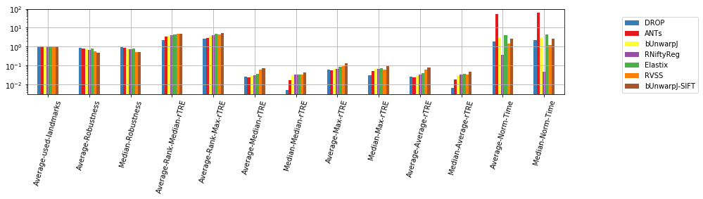
[11]:
dfx = pd.DataFrame(user_aggreg)[users_ranked].T[list(filter(lambda c: not c.startswith('STD-'), cols_general))]
ax = dfx.T.plot.bar(figsize=(len(cols_general) * 0.7, 4), grid=True, logy=True, rot=75, color=list_methods_colors(dfx.index))
# ax.legend(loc='upper center', bbox_to_anchor=(0.5, 1.35),
#           ncol=int(len(users) / 1.5), fancybox=True, shadow=True)
ax.legend(bbox_to_anchor=(1.1, 0.95))
ax.get_figure().tight_layout()
ax.get_figure().savefig(os.path.join(PATH_TEMP, 'bars_teams-scores.pdf'))
# plt.savefig(os.path.join(PATH_TEMP, 'fig_teams-scores.pdf'), constrained_layout=True)
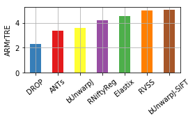
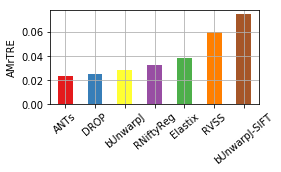
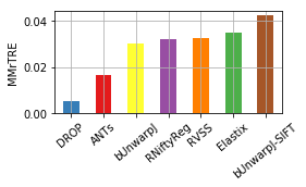
[12]:
for col, name in [('Average-Rank-Median-rTRE', 'ARMrTRE'),
                  ('Average-Median-rTRE', 'AMrTRE'),
                  ('Median-Median-rTRE', 'MMrTRE')]:
    plt.figure(figsize=(4, 2.5))
    dfx = pd.DataFrame(user_aggreg)[users_ranked].T[col].sort_values()
    ax = dfx.plot.bar(grid=True, rot=40, color=list_methods_colors(dfx.index))
    # ax = pd.DataFrame(user_aggreg).T.sort_values(col)[col].plot.bar(grid=True, rot=90, color='blue')
    _= plt.ylabel(name)
    ax.get_figure().tight_layout()
    ax.get_figure().savefig(os.path.join(PATH_TEMP, 'bar_teams-scores_%s.pdf' % col))
Transform the case format data to be simple form with extra colums for used and case ID to be able to draw a violine plot later.
[13]:
dfs_ = []
for usr in users:
    df = pd.DataFrame(user_cases[usr]).T
    df['method'] = usr
    df['case'] = df.index
    dfs_.append(df)
df_cases = pd.concat(dfs_).reset_index()
del dfs_

for col in df_cases.columns:
    try:
        df_cases[col] = pd.to_numeric(df_cases[col])
    except Exception:
        print('skip not numerical column: "%s"' % col)
# df_cases.head()
skip not numerical column: "name-tissue"
skip not numerical column: "type-tissue"
skip not numerical column: "name-reference"
skip not numerical column: "name-source"
skip not numerical column: "method"
Showing several distribution plots
[14]:
def _format_ax(ax, name, use_log=False, vmax=None):
plt.xticks(rotation=60)
if use_log:
ax.set_yscale('log')
if vmax:
ax.set_ylim([0, vmax])
ax.grid(True)
ax.set_xlabel('')
ax.set_ylabel(name)
ax.get_figure().tight_layout()
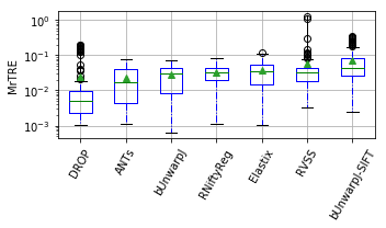
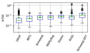
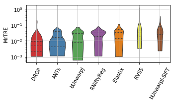
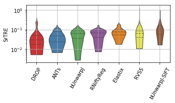
show_metrics = [('rTRE-Median', 'MrTRE', True, None, 0.01),
('rTRE-Max', 'SrTRE', True, None, 0.01),
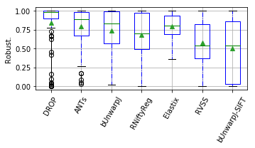
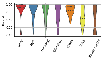
('Robustness', 'Robust.', False, None, 0.05),
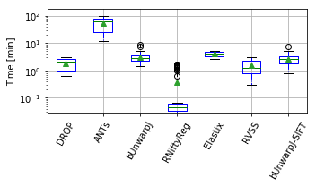
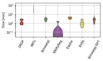
('Norm-Time_minutes', 'Time [min]', True, 180, 0.1)]
[15]:
for field, name, log, vmax, bw in show_metrics:
    # methods_ = list(dfg['method'].unique())
    vals_ = [df_cases[df_cases['method'] == m][field].values for m in users_ranked]
    df_ = pd.DataFrame(np.array(vals_).T, columns=users_ranked)
    fig, ax = plt.subplots(figsize=(5, 3))
    bp = df_.plot.box(ax=ax, showfliers=True, showmeans=True,
                      color=dict(boxes='b', whiskers='b', medians='g', caps='k'),
                      boxprops=dict(linestyle='-', linewidth=1),
                      flierprops=dict(linestyle='-', linewidth=1),
                      medianprops=dict(linestyle='-', linewidth=1),
                      whiskerprops=dict(linestyle='-.', linewidth=1),
                      capprops=dict(linestyle='-', linewidth=1),
                      return_type='dict')
    _format_ax(ax, name, log, vmax)
    ax.get_figure().savefig(os.path.join(PATH_TEMP, 'boxbar_teams-scores_%s.pdf' % field))
/home/jb/.local/lib/python3.6/site-packages/matplotlib/axes/_base.py:3477: UserWarning: Attempted to set non-positive ylimits for log-scale axis; invalid limits will be ignored.
  'Attempted to set non-positive ylimits for log-scale axis; '
[16]:
for field, name, log, vmax, bw in show_metrics:
    # methods_ = list(dfg['method'].unique())
    vals_ = [df_cases[df_cases['method'] == m][field].values for m in users_ranked]
    df_ = pd.DataFrame(np.array(vals_).T, columns=users_ranked)

    fig = plt.figure(figsize=(5, 3))
    # clr = sns.palplot(sns.color_palette(tuple(list_methods_colors(df_.columns))))
    ax = sns.violinplot(ax=plt.gca(), data=df_, inner="quartile", trim=True, cut=0., palette=COLOR_PALETTE, linewidth=1.)
    _format_ax(fig.gca(), name, log, vmax)
    fig.gca().grid(True)
    fig.savefig(os.path.join(PATH_TEMP, 'violin_teams-scores_%s.pdf' % field))
/home/jb/.local/lib/python3.6/site-packages/matplotlib/axes/_base.py:3477: UserWarning: Attempted to set non-positive ylimits for log-scale axis; invalid limits will be ignored.
  'Attempted to set non-positive ylimits for log-scale axis; '
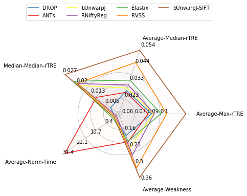
Visualise global results
[17]:
fields = ['Average-Max-rTRE', # 'Average-Max-rTRE-Robust',
          'Average-Median-rTRE', # 'Average-Median-rTRE-Robust',
          'Median-Median-rTRE', # 'Median-Median-rTRE-Robust',
          # 'Average-Rank-Max-rTRE', 'Average-Rank-Median-rTRE',
          'Average-Norm-Time', # 'Average-Norm-Time-Robust',
          'Average-Robustness',]
df = pd.DataFrame(user_aggreg)[users_ranked].T[fields]
df['Average-Weakness'] = 1 - df['Average-Robustness']
del df['Average-Robustness']

radar = RadarChart(df, fig=plt.figure(figsize=(5, 4)), colors=list_methods_colors(df.index), fill_alpha=0.02)
lgd = radar.ax.legend(loc='lower center', bbox_to_anchor=(0.5, 1.15), ncol=int(len(users) / 1.5))
radar.fig.savefig(os.path.join(PATH_TEMP, 'radar_teams-scores.pdf'),
                  bbox_extra_artists=radar._labels + [lgd], bbox_inches='tight')
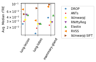
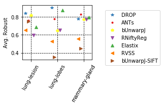
Visual statistic over tissue types
Present some statistis depending on the tissue types…
[18]:
cols_all = pd.DataFrame(user_aggreg).T.columns
col_avg_med_tissue = sorted(filter(
    lambda c: 'Median-rTRE_tissue' in c and not 'Rank' in c and 'Median-Median-' not in c, cols_all))
col_robust_tissue = sorted(filter(
    lambda c: 'Average-Robustness_tissue' in c and not 'Rank' in c, cols_all))
[19]:
params_tuple = [
    (col_avg_med_tissue, 'Avg. Median rTRE', 'Average-Median-rTRE__tissue_{}__All', True),
    (col_robust_tissue,'Avg. Robust', 'Average-Robustness__tissue_{}__All', False),
]

for cols, desc, drop, use_log in params_tuple:
    # print('"%s" with sample columns: %s' % (desc, cols[:3]))
    dfx = pd.DataFrame(user_aggreg)[users_ranked].T[cols]
    # colors = plt.get_cmap('nipy_spectral', len(dfx))
    fig, extras = draw_scatter_double_scale(
        dfx, colors=list_methods_colors(users_ranked), ax_decs={desc: None},
        idx_markers=list_methods_markers(users_ranked), xlabel='Methods', figsize=(2 + len(dfx.columns) * 0.95, 3),
        # legend_style=dict(bbox_to_anchor=(0.5, 1.15), ncol=4),
        legend_style=dict(bbox_to_anchor=(1.15, 0.95), ncol=1),
        x_spread=(0.4, 5))

    # DEPRICATED visualisation
    # ax = dfx.T.plot(style='X', cmap=plt.get_cmap('nipy_spectral', len(dfx)), figsize=(len(dfx) / 2 + 1, 5), grid=True)
    # ax.legend(loc='upper center', bbox_to_anchor=(1.2, 1.0), ncol=1)
    extras['ax1'].set_xticks(range(len(cols)))
    extras['ax1'].set_xticklabels(list(map(lambda c: col_metric_rename(c.replace(drop, '')), cols)), rotation=45, ha="center")
    _format_ax(extras['ax1'], desc, use_log, vmax=None)

    name = ''.join(filter(lambda s: s not in '(.)', desc)).replace(' ', '-')
    fig.savefig(os.path.join(PATH_TEMP, 'scat_teams-scores_tissue-%s.pdf' % name),
                bbox_extra_artists=(extras['legend'],), bbox_inches='tight')  #
[ ]: